2.1.2 Back Annotating a Schematic
Schematic back-annotation is the process of initializing the schematic to a known state. There are two ways to back annotate the schematic, both of which use 2.1.1 The Initial Conditions (.INIT) File.
To download the examples for Module 2, click Module_2_Examples.zip
In this topic:
Key Concepts
This topic addresses the following key concepts:
- There are two ways to back annotate a schematic:
- By writing the initial condition values to the schematic symbols.
- By including the contents of the initial conditions file in the simulation.
- The .INIT file which is created by SIMPLIS is overwritten every simulation run.
- Repeated initial condition statements for the same device will cause an error.
What You Will Learn
In this topic, you will learn the following:
- How to back annotate a schematic.
- How to initialize a schematic with a .INIT file.
- That included .INIT files override any schematic back annotation.
Getting Started
This topic uses the same schematic as the final section of 2.1.1 The Initial Conditions (.INIT) File.
Exercise #1: Schematic Back-Annotation
- If you have the .INIT file open, close the initial conditions file by clicking on the X toolbar icon, or with the menu .
- Close the waveform viewer, if it's open.
- Open the schematic 2.2_PFC_Critical_Conduction_Mode.sxsch.
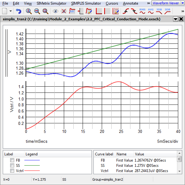
- Press F9 to run the simulation.Result: The waveform viewer opens with the simulation data plotted over the time interval of zero to 40ms.
- From the schematic menu, select
Result:
- The information in the .INIT file is parsed and the initial condition information is written to the individual symbols.
- A message is output to the command shell: Back annotation complete.
The next time the simulation is launched, the circuit will be in the same state as it was at time=40ms in this simulation.
Discussion
The method used in the Getting Started section is the most common way to back-annotate a schematic. The example circuit here is in soft-start operation, and the control voltages and the output voltage are ramping up from the starting values. A couple of items to note:
- The circuit uses a current source I2, capacitor C5, and PWL resistor R1 to effect soft-start. Because the capacitor is back-annotated, the simulation will pick up exactly where it left off. The back-annotation process effectively charges the capacitor to the voltage which it reached at the end of the previous simulation.
- The stop time for the example was strategically chosen to stop the simulation exactly on a line voltage zero crossing. Even though the sinusoidal input source V1 is excluded from back annotation, the voltage across V1 is zero every 20ms. This allows the circuit to continue simulating as if the voltage source was back-annotated.
- The PWL source V3 is set to zero, enabling the power supply. Because the source is effectively the same DC value for all simulation time, the fact that the source is not back-annotated doesn't impact the simulation results.
In the next exercise you will continue the simulation from this point, and observe the circuit is properly initialized.
Exercise #2: Run the Back-Annotated Circuit
You have already back-annotated the schematic, all you need to do is close the .INIT file (if the file is open) and run the simulation.
- If you have the .INIT file open, close the initial conditions file by clicking on the X toolbar icon, or with the menu .
- Press F9 to run the simulation.Result: The simulation starts at the back-annotated initial conditions. The waveform viewer now has two sets of waveforms - the first set from the initial simulation, and the second from the back-annotated simulation.
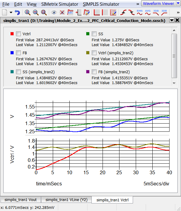
In the above graph it is easy to see that in the second simulation, the soft start voltage, SS starts at the same voltage where the first simulation stopped. In the next exercise you verify the measured voltage on the soft start capacitor is the same.
Exercise #3: Measure the Soft-Start Voltage
This schematic is setup to use fixed probe measurements for the three probes SS, Vctrl, and FB which measure the first and last values of the simulation vector. In this section you will verify that the starting voltages for the second simulation are the same as the final voltages for the first simulation.
- On the waveform viewer, note the green SS
curve from the first simulation has two measurement values:
- First Value=1.275V @ 0Secs
- Last Value=1.4384852V @40mSecs
- Next, look at the teal SS (simplis_tran2)
curve curve from the second simulation. This curve has the
following two measurement values:
- First Value=1.4384852V @40mSecs
- Last Value=1.6019602V @40mSecs
Although your measured value might be different from those above, the Last value from the initial simulation should match the First value from the last simulation.
Exercise #4: Initialize the Schematic by Including a .INIT File
SIMetrix/SIMPLIS has the ability to easily include text files in the simulation. The .INIT file is a sequence of SIMPLIS commands which tell the simulator to initialize each circuit device. Because the file is already in the correct format for SIMPLIS, all you need to do to initialize the circuit is to include the .INIT file with a .INCLUDE statement.
In this example you are going to include the auto-generated .INIT file. This means that each successive simulation will use the final values generated during the previous simulation. Each time you simulate, another two line cycles of soft-start will be displayed on the waveform viewer. To automatically include the init file,
- You first need to disable the initial conditions on the schematic. From the
schematic menu, select
Result: The schematic values for the initial conditions disappear.
- Select the schematic window and press F11 to open the command (F11) window.
- Scroll down to the bottom of the F11 window and add the following .INCLUDE
statement as the last line:
.INCLUDE ./SIMPLIS_Data/2.2_PFC_Critical_Conduction_Mode.deck.init
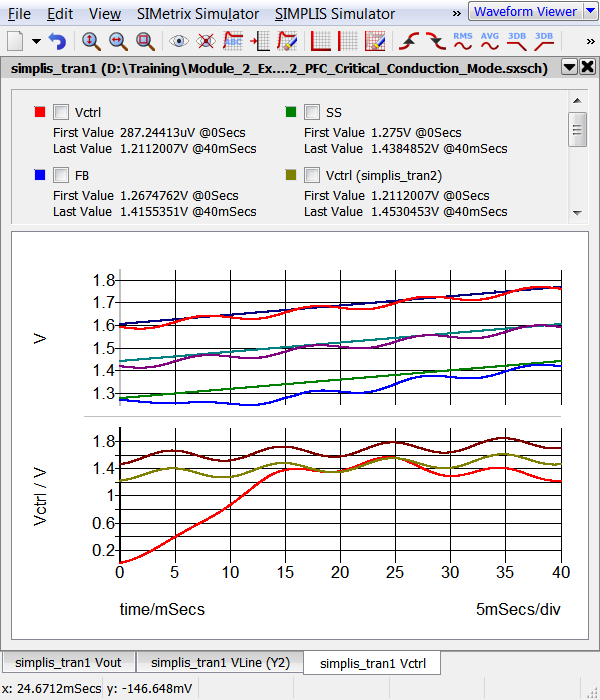
- Run the simulation. Result: The simulation starts from the initial conditions generated when the second simulation in exercise #2 finished. The waveform viewer shows three sets of curves:
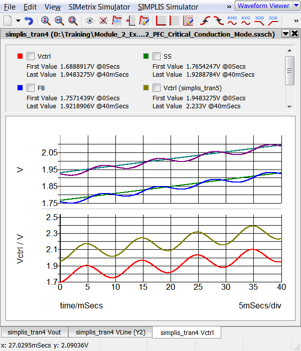
You can easily prove to yourself that each successive simulation continues where the last simulation left off. For example shown below is the results of the next two simulations. These were generated after closing the waveform viewer, so two sets of curves appear:
What Can Go Wrong?
The number of problems with loading initial conditions is quite small. By far the most common problem is when a circuit has duplicate or multiple initial condition statements for the same component. Each schematic symbol must be designed to handle initial conditions, and the method used by each symbol varies with the underlying device model. To avoid duplicate .INIT statements, you disabled the schematic back annotation when you included the .INIT file in the third exercise.
.INCLUDE ./SIMPLIS_Data/2.2_PFC_Critical_Conduction_Mode.deck.init
.INCLUDE ./SIMPLIS_Data/2.2_PFC_Critical_Conduction_Mode.deck.init
Conclusions and Key Points to Remember
- Back-annotation allows you to easily restart a simulation with initial conditions equal to the ending conditions of the previous simulation.
- The initial condition file in the SIMPLIS_Data directory is overwritten by each SIMPLIS POP or Transient simulation.