3.0 PFC Inductor Considerations

Key Concepts

This topic addresses the following key concepts:

• You must accurately set the fundamental frequency and wave shape for MDM post-processing to obtain correct inductor loss results.
• You must take care to determine whether the inductor waveforms are purely piecewise-linear (PWL), purely sinusoidal, or a mixture of sinusoidal and PWL, and also whether the sinusoidal component is rectified.
• Using more than one steady-state cycle for post-processing will provide the same results as using just one cycle, but will take longer.
• Post-processing takes longer when the waveforms are more complex.
• Just because an AC/DC converter is connected to the AC line voltage does not necessarily mean that the full line cycle is the inductor waveform steady-state cycle.
• It is your responsibility to ensure that the converter is in steady-state when you are running a transient simulation instead of a POP analysis.

What You Will Learn

In this topic, you will learn the following:

• What are the different types of wave shapes that MDM can recognize.
• How to properly set up MDM post-processing for an inductor of a PFC rectifier.

3.1 PFC Circuit and Inductor

Open the schematic 3.0_PFC_Critical_Conduction_Mode_with_MDM_Inductor.sxsch which is provided in the zip archive of examples you downloaded at the beginning of this tutorial. You will see the following circuit:

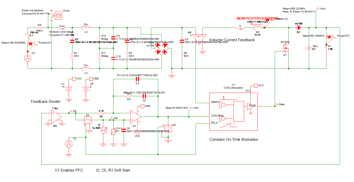
In this tutorial, you will focus on the inductor design for the PFC converter. The inductor design has already been provided and you will not modify it. The focus is only on correctly identifying the inductor fundamental frequency and wave shape of the inductor in order to properly set up and perform MDM post-processing.

You will notice in the above schematic that inductor L2 has been marked for MDM post-processing and therefore contains a Level 2 model. Double click the symbol L2.

Result: The Edit Multi-Level PWL Inductor dialog appears showing the following:

To examine the inductor model, click on Edit with SIMPLIS MDM....

Result: You will see an inductor designed using an EE32 with a custom gap of 0.2mm core made from the 3C81 material and 20 turns of trifilar Litz wire:

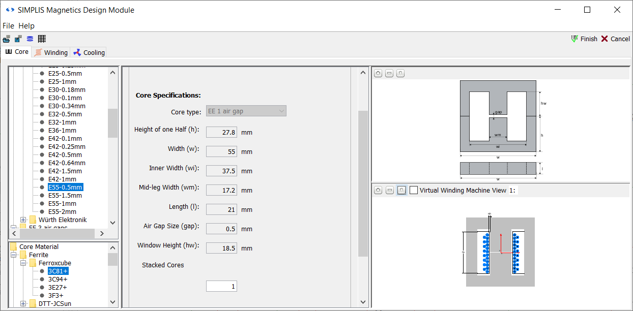
Click Cancel to close the main MDM window without making any changes to the magnetic design.

▲ back to top

3.2 Waveform Shapes Recognized by MDM

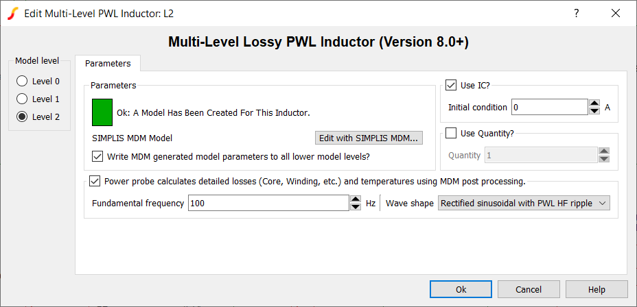
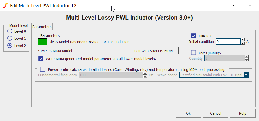
Double-click L2 to re-open the Edit Multi-Level PWL Inductor dialog.

Click on the down arrow in the Wave shape drop-down menu. You will see the following waveform shapes that you can select: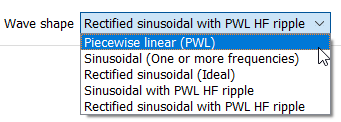

• Piecewise linear (PWL): use this when the inductor (or transformer) voltage, current, and flux density waveforms consist entirely of linear segments. You used this wave shape in the previous chapter for the Buck converter. This shape is typically encountered in non-resonant DC/DC converters (Buck, Boost, Buck-Boost, SEPIC, Ćuk, etc.).
• Sinusoidal (One or more frequencies): use this when the waveforms consist of several sinusoids imposed on one another, or if they are just a single ideal sinusoid. You will typically encounter such waveforms in EMI filters, resonant converters and of course many other circuits outside of switching converters.
• Rectified sinusoidal (Ideal): a single rectified sinusoid. Encountered for example as the output of a diode rectifier.
• Sinusoidal with PWL HF ripple: use this when the waveform has a lower frequency sinusoidal carrier (e.g. 50-100Hz) upon which a higher PWL switching waveform (e.g. in the kHz range) is superimposed. A type of waveform found in many AC/DC, DC/AC, and AC/AC converters.
• Rectified sinusoidal with PWL HF ripple: same as above, but with the sinusoidal carrier rectified. Found in many AC/DC converters.

What if your waveform does not neatly fit into any of the above categories? In that case, use Sinusoidal (One or more frequencies) as the fallback setting, as any waveform can be represented as a series of sinusoidal harmonics. You could have used that setting for example for the Buck converter in the previous chapter, instead of the PWL setting, but the core losses calculated would have been considerably less accurate.

▲ back to top

3.3 Determine the Inductor Waveform Shape and Frequency

Uncheck the Power probe calculates detailed losses... checkbox. You do NOT want to run MDM post-processing immediately. First you have to determine the fundamental frequency and wave shape. To do this you will initially run the simulation without post-processing. Click OK to close the dialog:

Press F9 to run the simulation. You will notice that this schematic is set up to perform a Transient analysis rather than the POP analysis that you performed in the previous chapter. When running a transient analysis, it is your responsibility to make sure that the simulation lasts long enough for the circuit to settle into steady-state.

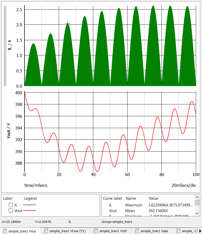
When the simulation finishes, select the simplis_tran1 Vout tab at the bottom of the Waveform Viewer. You will see that the inductor current (green) has settled into steady-state by the end of the simulation:

Now zoom in on the inductor current around a zero-crossing. Clearly you can see that the inductor current is a rectified sinusoidal waveform, with higher frequency PWL ripple:

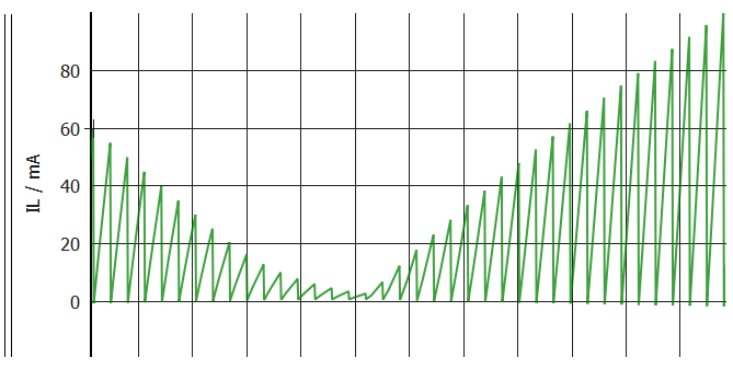
You can see that a PWL, high-frequency switching ripple is super-imposed on the sinusoidal carrier wave. Since the PFC rectifier is running in critical conduction mode, the current always decreases to zero before the next conversion cycle begins.

The AC line in this schematic has a frequency of 50Hz. Therefore you could set the fundamental frequency of the waveform as 50Hz - this would not be wrong. However, since the sine wave line voltage is rectified, the first and second half of the line cycle are the same as far as the inductor waveforms are concerned. Using 50Hz would produce correct results, but would needless repeat the same calculations twice. So, in this case, 100Hz can be used as the fundamental frequency.

To set now the schematic for MDM post-processing:

1. Double-click the symbol L2.
2. In the resulting dialog, check the Power probe calculates detailed losses... checkbox.
3. For the Fundamental frequency, enter 100.
4. For the Wave shape, select Rectified sinusoidal with PWL HF ripple.
5. Click OK.

▲ back to top

3.4 Run the Simulation and MDM Post-Processing

Press F9 to run the simulation. You will notice that MDM post-processing takes significantly longer than it took with the Buck converter. The pop-up dialog showing that MDM post-processing is in progress, may, depending on the speed of your machine, be displayed for about a minute:

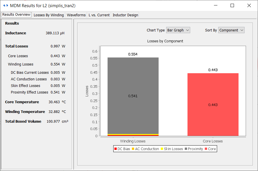
Finally the MDM Results window will appear:

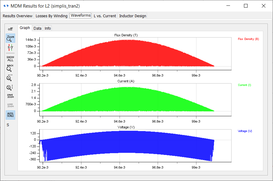
Switch to the Waveforms tab of the results window:

If you zoom in the flux density waveform you will see the PWL ripple:

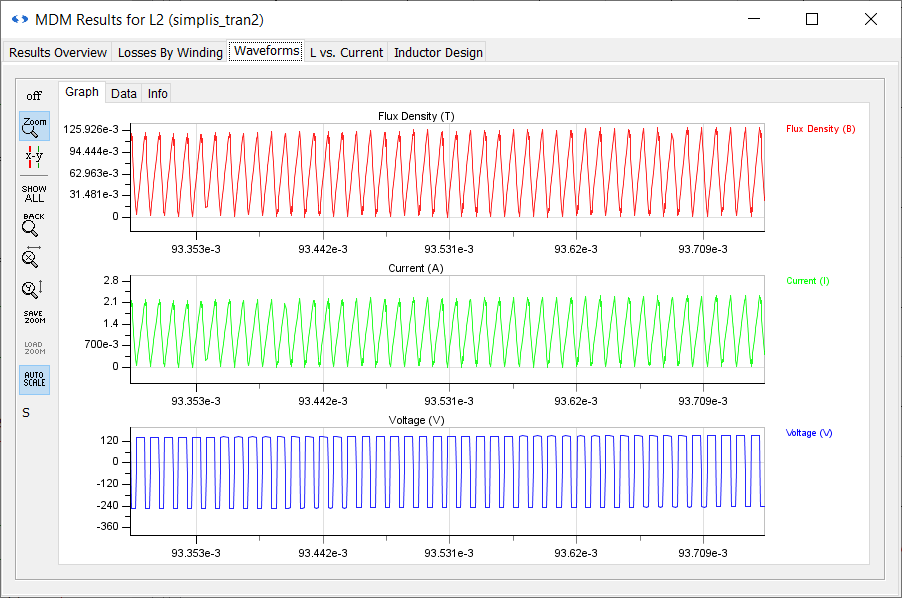
In order to accurately calculate core losses, MDM calculates the energy loss for each of these PWL flux segments and then averages the total over the 100Hz period to calculate the average power loss for the entire waveform. This is why the post-processing takes significantly longer than in the Buck converter, where the flux density waveform contains only two PWL segments. Therefore, the more complex and larger the waveform, the longer the post-processing will take.

You can now close this schematic and the MDM Results window. This concludes the treatment of inductors in this tutorial. You will now move to transformer design in the next chapter: 4.0 Flyback Converter Transformer Design

▲ back to top