Laplace Transfer Function
In this topic:
Overview
The Laplace transfer function device implements a linear device defined in the frequency domain by a Laplace transform. For example the Laplace transform ???MATH???\frac{1}{s+1}???MATH??? defines a first order low pass filter while ???MATH???exp(-s)???MATH??? defines a 1 second delay.
The SIMetrix Laplace transfer function device features two different methods of implementation, namely "lumped network" and "convolution". The lumped network implementation is fast and efficient and may be used for transfer functions that can be represented in polynomial form. The convolution method is more general purpose and can model a wide range of transfer functions. High performance is achieved by using a fast FFT-based convolution method.
User Interface
Selecting the menu
brings up the following dialog
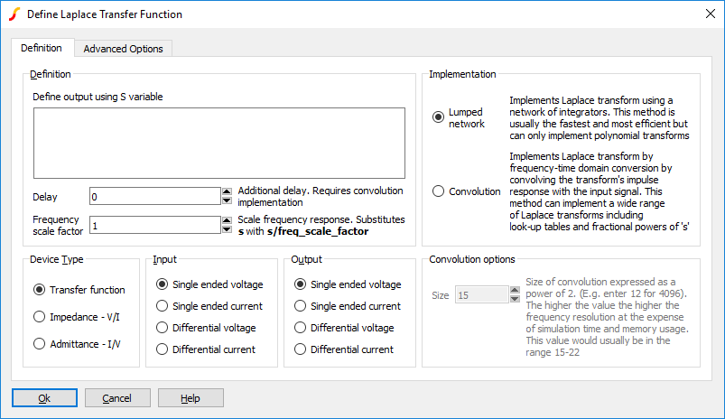 The operation of the various controls is described below.
| Definition | See Laplace expression | ||||||
| Delay | Adds delay in seconds. Requires convolution method. Equivalent to multiplying transfer functions by ???MATH???exp(-delay.s)???MATH??? | ||||||
| Frequency scale factor | Multiplier for frequency | ||||||
| Device type |
|
||||||
| Input | Input configuration for transfer function | ||||||
| Output | Output configuration for transfer function | ||||||
| Implementation | See Implementation | ||||||
| Convolution Options | Convolution size. Increase this value to increase the upper frequency limit. This will slow down the simulation and increase memory consumption. Memory usage for a single device is approximately ???MATH???96*2^N???MATH??? bytes where ???MATH???N???MATH??? is the value entered here. Note that memory is partly shared for multiple devices. The upper frequency is of the order of ???MATH???2^{N-1}/T???MATH??? where T is the simulation time. So for example, with a simulation time of 1ms and N=15, the upper frequency limit will be in the region of 16MHz. Higher frequencies will be gradually attenuated. As well as increasing memory consumption, higher values of convolution size will slow the simulation. This does not become significant until N exceeds about 17 to 18 but increases markedly for higher values. |
The Advanced Options tab displays the following:
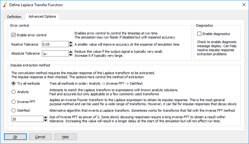
| Error control | Configures time-step control algorithm. For rapidly changing inputs the time step must be kept small to retain good accuracy. The parameters entered here control this mechanism. | ||||||||||
| Diagnostics | Check box to enable some diagnostic run-time messages. These provide information on the extraction of the impulse response. | ||||||||||
| Impulse extraction method |
Parameters controlling extraction of the impulse response.
|
Laplace Expression
The Laplace expression defines the behaviour of the device in the frequency domain. For example '1/(s+1)', defines a simple single pole low-pass filter. The expression may contain arithmetic operators and a number of functions as described in the following sections. Be aware that not any expression is physically realisable; for example 'exp(s)' defines a negative delay, that is a device whose output responds to an input in the future.
Operators
+ - * / ^where ^ means raise to power. For lumped network implementation, the power must be an integer. Non-integral powers may be entered for convolution implementation.
Constants
Any decimal number following normal rules. SPICE style engineering suffixes are accepted.
s Variable
This can be raised to a power using ^, for example s^2. If the power is an integer between 0 and 9 the ^ may be omitted. For example: s2 is the same as s^2.
Functions
| Function Syntax | Description |
| sqrt(x) | ???MATH???\sqrt{x}???MATH??? |
| exp(x) | ???MATH???e^{x}???MATH??? |
| ln(x) | ???MATH???\log_e(x)???MATH??? |
| log10(x) | ???MATH???\log_{10}(x)???MATH??? |
| sin(x) | ???MATH???\sin(x)???MATH??? |
| cos(x) | ???MATH???\cos(x)???MATH??? |
| tan(x) | ???MATH???\tan(x)???MATH??? |
| acos(x) | ???MATH???\cos^{-1}(x)???MATH??? |
| asin(x) | ???MATH???\sin^{-1}(x)???MATH??? |
| atan(x) | ???MATH???\tan^{-1}(x)???MATH??? |
| sinh(x) | ???MATH???\sinh(x)???MATH??? |
| cosh(x) | ???MATH???\cosh(x)???MATH??? |
| tanh(x) | ???MATH???\tanh(x)???MATH??? |
| asinh(x) | ???MATH???\sinh^{-1}(x)???MATH??? |
| acosh(x) | ???MATH???\cosh^{-1}(x)???MATH??? |
| atanh(x) | ???MATH???\tanh^{-1}(x)???MATH??? |
| atan2(x,y) | ???MATH???\tan^{-1}(\frac{y}{x})???MATH??? |
| pow(x,y) | ???MATH???x^y???MATH??? |
Filter response functions
Filter response functions may be used in both lumped network implementation and convolution implementation.
These are described in the following table:
| Function Syntax | Filter Response |
| BesselLP(order, cut-off) | Bessel low-pass |
| BesselHP(order, cut-off) | Bessel high-pass |
| ButterworthLP(order, cut-off) | Butterworth low-pass |
| ButterworthHP(order, cut-off) | Butterworth high-pass |
| ChebyshevLP(order, cut-off, passband_ripple) | Chebyshev low-pass |
| ChebyshevHP(order, cut-off, passband_ripple) | Chebyshev high-pass |
| order | Integer specifying order of filter. There is no maximum limit but in practice orders larger than about 50 tend to give accuracy problems. |
| cut-off | -3dB Frequency in Hertz. |
| passband_ripple | Chebyshev only. Passband ripple spec. in dB. |
Lookup tables
The frequency response of a system may be defined in tabular form using lookup tables. The lookup table consists of a sequence of values arranged in triplets. Each triplet is in the form ???MATH???frequency, value1, value2???MATH??? where ???MATH???value1???MATH??? and ???MATH???value2???MATH??? define the magnitude and phase in various ways as described below.
There are five variants of the lookup table as described below:
| Function Name | value1 | value2 |
| Table | dB | phase in degrees |
| Table_M | magnitude | phase in degrees |
| Table_R | dB | phase in radians |
| Table_MR | magnitude | phase in radians |
| Table_RI | real part | imaginary part |
Example
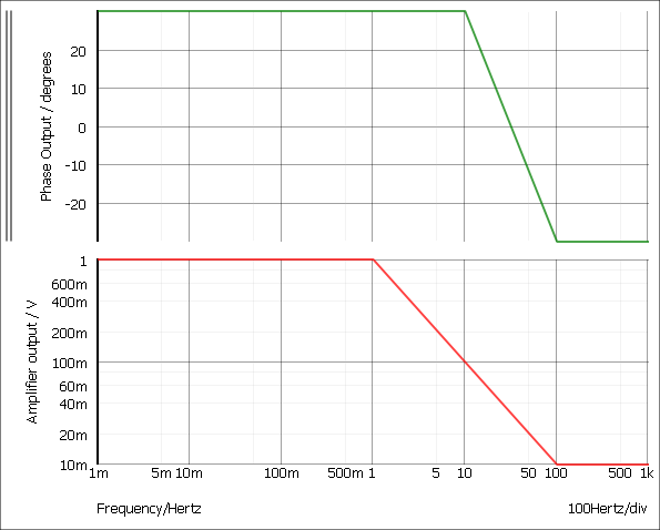
Table_M(0.01,1,30, 1,1,30, 10,0.1,30, 100,0.01,-30)
The above defines a response with a gain of 1 and a phase shift of 30 degrees from 0.01Hz to 1Hz. From 1Hz to 10Hz the gain falls from 1 to 0.1 with the phase shift remaining at 30 degrees. From 10Hz to 100Hz the gain falls from 0.1 to 0.01 and the phase changes from 30 to -30 degrees.
In real life it is not possible to implement a characteristic with the above behaviour as it is non-causal. However, it can be implemented if a suitable delay is added to the characteristic. The delay may be added in the Define Laplace Transfer Function dialog box in the Definition section - see the Delay entry. Alternatively it may be added to the Laplace expression using ???MATH???exp(-delay.s)???MATH???. E.g:
Table_M(0.01,1,30, 1,1,30, 10,0.1,30, 100,0.01,-30) * exp(-s*2)
The above adds a 2 second delay.
For ease of reading, each triplet in the table may be placed on a separate line by prefixing each line with a '+' character. E.g.
Table_M(
+ 0.01,		1,		30,
+ 1,		1,		30,
+ 10,		0.1,		30,
+ 100,		0.01,		-30)
Interpolation Between defined frequency points, the Laplace transfer function finds the magnitude and phase using interpolation. The interpolation is performed logarithmically on the magnitude data. Values outside the table frequency range are defined by their respective end points.
For the above example the magnitude and phase are shown below:
Parameters
Parameters (defined with .PARAM) may be used in Laplace expressions but currently only if convolution implementation is selected.
For the lumped network implementation you can use parameters in the underlying simulator device if you define the expression in terms of the numerator and denominator coefficients. Refer to the S-domain Transfer Function Block in the Simulator Reference Manual for further details.
Device type
| Transfer function | Expression defines output/input. |
| Impedance V/I | Two terminal device, expression defines voltage/current. |
| Admittance I/V | Two terminal device, expression defines current/voltage. |
Implementation
| Lumped network | The Laplace transform is implemented using a network of integrators. |
| Convolution | The Laplace transform is implemented by convolving the impulse response of the Laplace transform with the input signal. |
Lumped Network
The diagram below shows the configuration used for a third order network.
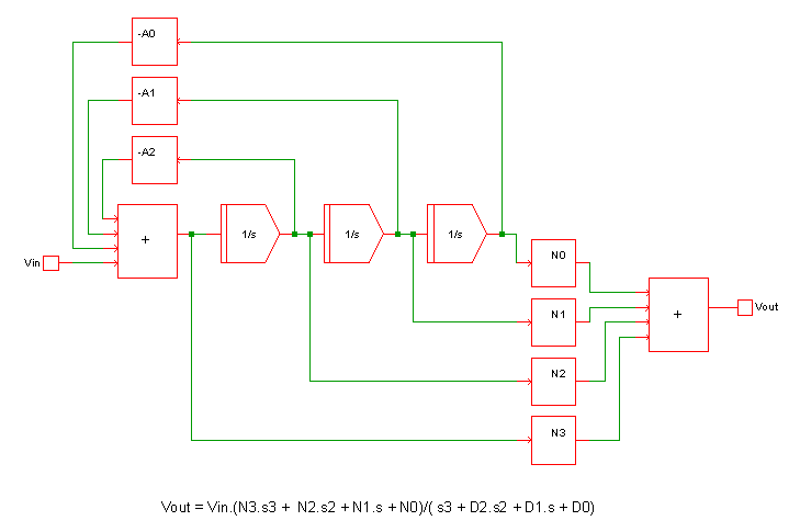 This method can implement a quotient of polynomials in the s variable and any expression that can be reduced to a quotient of polynomials. For such expressions it is fast and efficient.
This method cannot implement expressions containing arbitrary functions such as square-root or exponentials. Such Laplace expressions must be implemented using the convolution method.
Convolution
This is a general purpose method and can implement a wide range of Laplace transforms.
In the frequency domain, a linear system may be represented by: \[ Vout(s) = Vin(s).f(s) \] where ???MATH???f(s)???MATH??? is the transfer function.
In the time domain the same system may be represented by: \[ Vout(t) = Vin(t) \ast f(t) \] Where ???MATH???f(t)???MATH??? is the impulse response of ???MATH???f(s)???MATH??? and ???MATH???\ast???MATH??? is the convolution operator.
This method is challenging to implement as simple convolution applied to simulation data in its raw form is an ???MATH???\mathcal{O}(n^2)???MATH??? algorithm. This means that the number of computations required at each step is proportional to the square of the number of steps. In practice this becomes unacceptably slow when there are more than about 10000 time steps.
SIMetrix overcomes this performance limitation by using an FFT based fast convolution method with a computation speed of ???MATH???\mathcal{O}(n\log{}^2n)???MATH???. Although dramatically faster, this algorithm requires data to be presented to it at fixed-interval steps which has the effect of placing an upper frequency limit. The actual upper frequency limit can be arbitrarily increased by increasing the number of steps (the value of ???MATH???n???MATH???) at the expense of speed and the memory consumed. In practice the default settings work well in most applications and give good performance and accuracy.
| Analytical | Matches the Laplace transform to known analytical solutions. For example ???MATH???\frac{1}{\sqrt{}(s)}???MATH??? has the impulse response of ???MATH???\frac{1}{2.\pi\sqrt{t}}???MATH???. SIMetrix will automatically detect this and other known Laplace transforms. |
| Inverse FFT | Calculates the inverse Fourier transform of the Laplace expression. This is a general purpose method that can be applied to a wide-range of Laplace transforms. However, it has the condition that the impulse response must decay to zero during the time interval. |
| Stehfest method | A method to calculate the inverse Laplace transform. Sometimes this method works for slowly decaying transforms that fail with the inverse FFT method. |
Impulse Response
Problems with Impulse Response Extraction
For the convolution method an impulse response of the Laplace transfer function must be extracted. As mentioned above, three methods are attempted. The inverse FFT method and Stehfest methods are approximate in nature and for this reason, the result from each method is tested. If the test fails the impulse response is rejected and another method is attempted. If all methods fail the simulation will abort.
Transfer functions that decay slowly are likely to fail the inverse FFT method as this method requires that the impulse response decay to zero or nearly to zero. If the Stehfest method also fails, the problem can sometimes be resolved by increasing the inverse FFT size. This increases the duration over which the inverse FFT is evaluated so providing a longer time to decay.
In many situations the impulse response extraction fails because the transfer function is non-causal. This means that it has a response in negative time. Non-causal transfer functions can be made causal by adding a delay.
Impulse Response Cache
The impulse response is cached to speed up subsequent simulations with the same response. The cache is located here:
C:\Users\<login-name>\AppData\Roaming\SIMetrix Technologies\SIMetrix810\LaplaceCache
where <login-name> is the name used to log in to your system. This can be deleted at any time. The cache is size limited to 250Mbytes by default. This can be changed using the option variable LaplaceCacheSizeMBytes. Type 'Set LaplaceCacheSizeMBytes=nnn' at the command line to set a new value.
Impulse Response Analytical Extraction
The impulse response analytical extraction attempts to match the transfer function to one of the following patterns. The parameters ???MATH???a???MATH???, ???MATH???b???MATH???, ???MATH???c???MATH??? etc represent constant values.
| Laplace expression | Impulse response |
| ???MATH???a???MATH??? | ???MATH???a.\delta(t)???MATH??? |
| ???MATH???a/(b.s)???MATH??? | ???MATH???a/b???MATH??? |
| ???MATH???a/\sqrt{b.s}???MATH??? | ???MATH???a/\sqrt{2.\pi.b.t}???MATH??? |
| ???MATH???a/(b.s+c)???MATH??? | ???MATH???a/b.e^{-c/b.t}???MATH??? |
| ???MATH???a/\sqrt{b.s+c}???MATH??? | ???MATH???a*e^{-c.t/b}/\sqrt{b.\pi.t}???MATH??? |
| ???MATH???\sqrt{a/(b.s+c)}???MATH??? | ???MATH???\sqrt{a}*e^{-c.t/b}/\sqrt{b.\pi.t}???MATH??? |
| ???MATH???{\displaystyle \frac{a}{b.s^2+c.s+d}}???MATH??? | ???MATH???{\displaystyle \frac{-(e^{-t/2(\sqrt{p^2-4q}+p)}-e^{t/2(\sqrt{p^2-4q}-p)}}{\sqrt{p^2-4q}}}???MATH??? ???MATH???p=c/b???MATH??? and ???MATH???q=d/b???MATH??? |
| ???MATH???a.e^{b.s}???MATH??? | ???MATH???a.\delta(b+t)???MATH??? |
| ???MATH???a/(b.s^c)???MATH??? | ???MATH???{\displaystyle \frac{a.t^{c-1}}{b.\Gamma(c)}}???MATH??? |
| ???MATH???{\displaystyle \frac{a.s^2+b.s+c}{d.s^2+g.s+f}}???MATH??? | ???MATH???{\textstyle [\frac{-(e^{t.arg2}-e^{t.arg3})*(-p.u+2q+u^2-2v)}{2arg1} - \frac{ (u-p)(e^{t.arg2}+e^{t.arg3}) }{2}+\delta(t)]\frac{a}{d}}???MATH??? ???MATH???p = b/a???MATH??? ???MATH???q = c/a???MATH??? ???MATH???u = g/d???MATH??? ???MATH???v = f/d???MATH??? ???MATH???arg1 = \sqrt{u^2-4v}???MATH??? ???MATH???arg2 = -arg1/2-u/2???MATH??? ???MATH???arg3 = arg1/2-u/2???MATH??? |
| ???MATH???{\displaystyle \frac{a.s+b}{c.s^2+d.s+f}}???MATH??? | ???MATH???{\displaystyle \frac{a}{c}.\frac{(2q-u)(arg2 - arg3) + \sqrt{u^2-4v}(arg3 + arg2)}{2\sqrt{u^2-4v}}}???MATH??? ???MATH???q = b/a???MATH??? ???MATH???u = d/c???MATH??? ???MATH???v = f/c???MATH??? ???MATH???arg2 = e^{t.(\sqrt{u^2-4v}/2-u/2)}???MATH??? ???MATH???arg3 = e^{t.(-\sqrt{u^2-4v}/2-u/2)}???MATH??? |
| ???MATH???{\displaystyle \frac{a.s+b}{c.s+d}}???MATH??? | ???MATH???{\displaystyle \frac{e^{-d.t/c}(b.c-a.d)}{c^2}+\frac{a.\delta(t)}{c}}???MATH??? |
| ???MATH???{\displaystyle \frac{\sqrt{a.s+b}}{\sqrt{c.s+d}}} ???MATH??? | ???MATH???(\alpha.(I1(\alpha.t)-I0(\alpha.t)) + \delta(t)).e^{-\beta.t}.Y???MATH??? ???MATH???Y = \sqrt{a/c}???MATH??? ???MATH???\alpha = (d/c-b/a)/2???MATH??? ???MATH???\beta = (d/c+b/a)/2???MATH??? I0 and I1 are Bessel functions |
The analytic matching algorithm will attempt to match partial expressions as well as the whole expression if they are combined by addition, subtraction or multiplication. For example:
???MATH???(1/(s+1))*exp(-s)???MATH???
will be matched to the product of ???MATH???1/(s+1)???MATH??? and ???MATH???exp(-s)???MATH???. Respectively these have impulse responses of ???MATH???e^{-t}???MATH??? and ???MATH???\delta(1+t)???MATH??? and those two impulse responses will be convolved to yield the final result. Note that this only succeeds if all partial expressions can be matched analytically.
To exploit this method, ensure that the expression is entered in a manner that keeps each partial expression distinct. For example, the following would be matched correctly:
???MATH???1/(s+1)*1/(s+2)???MATH???
as this would be seen as the two partial expressions ???MATH???1/(s+1)???MATH??? and ???MATH???1/(s+2)???MATH??? each of which can be resolved analytically. The final result would be obtained by convolving the two impulse responses.
However the following mathematically identical expression would not be matched:
???MATH???1/((s+1)*(s+2))???MATH???
The analysis algorithm does not attempt to decompose denominator products so this will not be recognised analytically. The above would be extracted using inverse FFT which would usually be successful but might not be if the run time is considerably shorter than the time constant.
| ◄ Non-linear Transfer Function | Device Library and Parts Management ▶ |