Generating Efficiency Plots with Multi-Step Runs in DVM
In the previous section, DVM Principles, you learned the principles of DVM, including a few basic testplan entries. In this topic you will learn how to use other testplan entries to customize the output from a testplan. These additional testplan entries are used in the built-in efficiency testplan.
To download the examples for the Applications Module, click Applications_Examples.zip
In this topic:
Key Concepts
- You can change symbol properties with a LoadComponentValues entry in the testplan. To use this testplan entry, you define the component reference designators, property names, and their new property values in a text file. In the testplan, you enter the path to that file. DVM loads the schematic with the property values just as if you ran the and selected the filename in the testplan field.
- The Alias() entry allows you to duplicate scalar values, effectively creating new categories of scalar values. In this topic, you will create groups of measured efficiency, one group per input voltage.
- Multi-Step simulations, even when run on a single core, are much faster than single step simulations because the schematic is prepared for simulation once.
- When you add Multi-Core to your Multi-Step simulations using a Pro or Elite license, you will see a dramatic reduction in the time it takes to complete your simulations.
- The CreateXYScalarPlot() function is an extremely powerful function which plots measured values against measured values. In these exercises, you will plot efficiency on the y-axis vs. the load current on the x-axis for three different input voltages.
What You Will Learn
In this topic, you will learn the following:
- How to change properties of multiple symbols, including the DVM Control Symbol using the LoadComponentValues testplan entry.
- How to create scalar aliases using the Alias() testplan entry.
- How to plot scalars vs. scalars on an X-Y plot using the CreateXYScalarPlot() function.
Getting Started
To get started, open the schematic apps_d_1_llc_converter_efficiency.sxsch. This schematic is prepared to run DVM as described in the DVM Principles topic.
Exercise #1: Create And Run The Built-In Efficiency Testplan
Once you have a schematic configured for DVM with DVM sources, loads, and a control symbol, you can use the menu to create a testplan which generates efficiency curves vs. load current for up to three input voltages. This menu item creates a testplan customized for the schematic, reading the numeric specifications from the DVM control symbol for input voltage and output load. To create this testplan for the apps_d_1_llc_converter_efficiency.sxsch schematic:
- From the schematic view, select the menu.Result: The Configure Efficiency Testplan dialog appears:
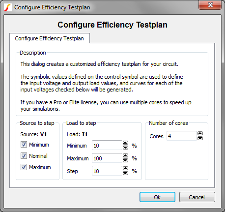
- The default configuration runs 10 load current steps and three input voltage
steps, for a total of 30 simulation steps. The program defaults to use the maximum
number of cores your machine or license is limited to. Click Ok to create a
testplan with the default values.Result: When you accept this dialog, the program reads the numeric values for the minimum, nominal, and maximum input source voltage, and the 100% load current value. A multi-step test is created for the schematic using these numeric values. After the program creates this testplan, you will be prompted to save the testplan with a file selection dialog. You can use the default name and click Ok.
- After you save the testplan, the test selection dialog appears:
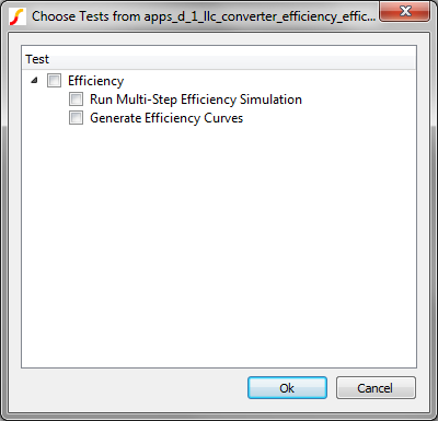
- Check the first box in the dialog, to the left of the Efficiency text.
Both tests in the testplan will be automatically selected.
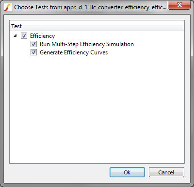 and Click Ok.Result: DVM runs the two tests in sequence. The first test runs a nested multi-step simulation to generate the measured efficiency values. The second test doesn't run the simulator, rather it plots the efficiency on the y-axis, and the load current on the x-axis, using the data generated in the first test.
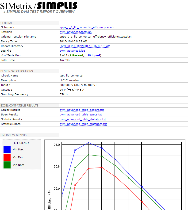
In this exercise, you generated a testplan using the built-in efficiency testplan generator. This menu item actually creates three files - a testplan, and two LoadComponentValues files. In the next exercise, you will learn the additional testplan syntax required to generate the efficiency curves.
Exercise #2: Examine the Built-In Efficiency Testplan
In this exercise, you will learn what testplan syntax was used to generate the efficiency curves using the built-in efficiency testplan generator. As you will see, only a handful of new testplan entries are used, but with dramatic results.
| 1 | *** auto-created testplan : apps_d_1_llc_converter_efficiency_efficiency.testplan | ||||||||
|---|---|---|---|---|---|---|---|---|---|
| 2 | *** schematic name: apps_d_1_llc_converter_efficiency.sxsch | ||||||||
| 3 | *** date: 10/16/2018 | ||||||||
| 4 | *** time: 8:19 AM | ||||||||
| 5 | *** | ||||||||
| 6 | *** input parameters: | ||||||||
| 7 | *** input voltages for (V1) : | ||||||||
| 8 | *** Minimum: 360V | ||||||||
| 9 | *** Nominal: 380V | ||||||||
| 10 | *** Maximum: 400V | ||||||||
| 11 | *** | ||||||||
| 12 | *** output loads for (I1) in percent of full load: | ||||||||
| 13 | *** 10, 20, 30, 40, 50, 60, 70, 80, 90, 100 | ||||||||
| 14 | *** | ||||||||
| 15 | *** using (4) cores | ||||||||
| 16 | *** | ||||||||
| 17 | *** a total of (30) steps will be run. | ||||||||
| 18 | *?@ LoadComponentValues | Analysis | Objective | Label | Create | Create | Create | Create | |
| 19 | lcv\apps_d_1_llc_converter_efficiency_efficiency_change.compvalues.txt | Multi-Step | Steady-State | Efficiency|Run Multi-Step Efficiency Simulation | Alias(Efficiency,Efficiency_%V1_VALUE%) | ||||
| 20 | lcv\apps_d_1_llc_converter_efficiency_efficiency_reset.compvalues.txt | NoSimulation | Efficiency|Generate Efficiency Curves | CreateXYScalarPlot( AVG(ILOAD), Efficiency_360, AVG(ILOAD) Efficiency_360, DVM Vin Min, DVM Efficiency , A1, vert, usescalars=multi xlabel=Load Current xunits=A ylabel=Efficiency yunits=%%% showpoints=true color=red ) | CreateXYScalarPlot( AVG(ILOAD), Efficiency_380, AVG(ILOAD) Efficiency_380, DVM Vin Nom, DVM Efficiency , A1, vert, usescalars=multi xlabel=Load Current xunits=A ylabel=Efficiency yunits=%%% showpoints=true color=green ) | CreateXYScalarPlot( AVG(ILOAD), Efficiency_400, AVG(ILOAD) Efficiency_400, DVM Vin Max, DVM Efficiency , A1, vert, usescalars=multi xlabel=Load Current xunits=A ylabel=Efficiency yunits=%%% showpoints=true color=blue ) | PromoteGraph( DVM Efficiency , 1 ) |
The Multi-Step Test (Row #19)
lcv\apps_d_1_llc_converter_efficiency_efficiency_change.compvalues.txt
The LoadComponentValues Entry
| 1 | *** | ||
|---|---|---|---|
| 2 | *** change LoadComponentValues file for testplan : apps_d_1_llc_converter_efficiency_efficiency.testplan | ||
| 3 | *** | ||
| 4 | DVM_CONTROL.ANALYSIS_MULTI_STEP_PARAM_NAME | V1_VALUE;I1_VALUE | |
| 5 | DVM_CONTROL.ANALYSIS_MULTI_STEP_LIST_VALUES | 360,380,400;10,20,30,40,50,60,70,80,90,100 | |
| 6 | DVM_CONTROL.ANALYSIS_MULTI_STEP_NUM_CORES | 4 | |
| 7 | DVM_CONTROL.ANALYSIS_MULTI_STEP_STEP_TYPE | LIST;LIST | |
| 8 | *** | ||
| 9 | *** | ||
| 10 | V1.DC_VOLTAGE | {V1_VALUE} | |
| 11 | *** | ||
| 12 | I1.DC_CURRENT | {I1_VALUE*0.01*5} | |
| 13 | I1.LOAD_RESISTANCE | {24/(I1_VALUE*0.01*5)} |
- V1_VALUE
- I1_VALUE
{24/(I1_VALUE*0.01*5)}
This
expression is simply the nominal output voltage (24V) divided by the stepped
load current in percent (I1_VALUE) times the nominal, full load current (5A.) The Create Testplan Entry
Alias(Efficiency,Efficiency_%V1_VALUE%)This Alias() entry creates groups of scalars based on the stepped input voltage value. How this works is relatively simple - after the multi-step simulation runs, there are 30 measured scalar values for the converter efficiency - each one with the same name: Efficiency. What this alias entry does is take these scalar values and make duplicates with the %V1_VALUE% text replaced with the actual stepped parameter value for V1_VALUE. In this example, the input voltage is stepped over three values and the following scalars are aliased:
- Efficiency_360
- Efficiency_380
- Efficiency_400
The other entries in the first test tell the program to run a Multi-Step analysis (introduced in 3.1 SIMPLIS Multi-Step Analysis), and to run a SteadyState Test Objective.
Order Of Operations
It is important to note the order of operations in the above test row. The LoadComponentValues entry comes before (to the left) of the Analysis: Multi-Step entry. This is an extremely important concept: DVM processes entries in left-to-right order, so in this case, you need to put the LoadComponentValues entry to the left of the Multi-Step entry. This is because the Multi-Step entry reads the DVM Control Symbol properties, setting the circuit up for a multi-step simulation.
The Final Test
The final test isn't really much of a test at all. This test uses the NoSimulation entry in the analysis column. This tells the program to not launch a simulation, and instead process the other columns in the testplan.
- To reset the schematic component values back to the values present when the testplan was generated
- Generate the x-y plots of efficiency vs. load current.
The LoadComponentValues Entry
{RLOAD}
| 1 | *** | ||
|---|---|---|---|
| 2 | *** reset LoadComponentValues file for testplan : apps_d_1_llc_converter_efficiency_efficiency.testplan | ||
| 3 | *** | ||
| 4 | DVM_CONTROL.ANALYSIS_MULTI_STEP_PARAM_NAME | ||
| 5 | DVM_CONTROL.ANALYSIS_MULTI_STEP_LIST_VALUES | ||
| 6 | DVM_CONTROL.ANALYSIS_MULTI_STEP_NUM_CORES | 1 | |
| 7 | DVM_CONTROL.ANALYSIS_MULTI_STEP_STEP_TYPE | LIN | |
| 8 | *** | ||
| 9 | *** | ||
| 10 | V1.DC_VOLTAGE | {VIN} | |
| 11 | *** | ||
| 12 | I1.DC_CURRENT | 500m | |
| 13 | I1.LOAD_RESISTANCE | {RLOAD} |
The Create Testplan Entries
There are four Create testplan entries for the final test. The first three each contain a single CreateXYScalarPlot() entry, these three entries create a single x-y curve for the converter efficiency. Three entries are needed to create the curves for the three input voltages.
The syntax for the CreateXYScalarPlot() function can be found at the hyperlink above and is too detailed to be covered in this topic.
The final Create testplan entry "promotes" or makes a copy of the efficiency curves and places this copy on the overview report. It is this copy that you saw at the end of the first exercise.
Conclusions and Key Points to Remember
- Using the Multi-Step analysis on two stepped parameters in DVM allows you to quickly analyze a circuit's performance over line and load variations.
- Applying Multi-Core capability to the simulation results in even faster simulation times.
- The CreateXYScalarPlot() function generates X-Y plots from previously generated scalar values. This function saves time by automatically plotting the scalar results.